23 Double integrals in polar coordinates
Polar coordinates
The Cartesian coordinates \((x,y)\) become needlessly complex with respect to some basic double integrals, namely those over discs and other circular regions. The polar coordinates \((r,\theta)\), which we review here, are a more natural choice for such integrals.
- \(r\) measures the distance between a point and the origin, so we have \[ r = \sqrt{x^2 + y^2}. \]
- \(\theta\) measures the (counterclockwise) angle from the positive x-axis, and thus \[ x \tan \theta = y. \]
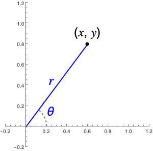
We can recover Cartesian coordinates from polar coordinates using \[ x = r \cos \theta \quad \text{and} \quad y = r \sin \theta. \]
In addition to reviewing the unit circle, this unit benefits from recalling the double angle formulas, \[ \cos(2\theta) = \cos^2(\theta) - \sin^2(\theta) \quad \text{and} \quad \sin(2\theta) = 2 \sin(\theta) \cos(\theta), \] and the power reduction formulas, \[ \cos^2(\theta) = \frac{1 + \cos(2\theta)}{2} \quad \text{and} \quad \sin^2(\theta) = \frac{1 - \cos(2\theta)}{2}. \]
To see how useful polar coordinates can be, consider a double integral over the annulus of inner radius \(1\) and outer radius \(2\) centered at the origin. In Cartesian coordinates, the inner circle is defined by the implicit equation \(x^2 + y^2 = 1\), and the outer circle by \(x^2 + y^2 = 4\). In polar coordinates, the inner circle is simply \(r = 1\) and the outer circle \(r = 2\). This is already nice, but consider how much simpler the slicing becomes:
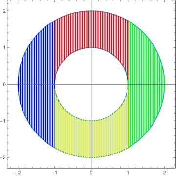
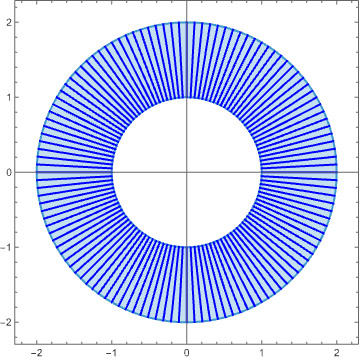
Note how the polar slices spread out as we move away from the origin. More on that later.
Curves in polar coordinates
Just as we are used to studying plots of the form \(y = f(x)\) in Cartesian coordinates, we can consider relationships between \(r\) and \(\theta\) in polar coordinates. We are especially interested in functions of the form \(r = f(\theta)\), which describe curves whose distance from the origin varies with angle off the horizontal axis. When describing these curves, it is often useful to specify permissible values of \(\theta\).
We have already seen that this is a circle of constant radius \(1\); as \(\theta\) varies, we trace out the circle once. Compare this with what it takes to specify the circle in Cartesian coordinates, where we have to write \(y = \sqrt{1-x^2}\) and \(y = -\sqrt{1-x^2}\) to define the top and bottom halves (note that \(x\) varies from \(-1\) to \(1\)).
Rather than plotting along the \(x\)-axis, we wrap the curve around the origin according to the angle \(\theta\).
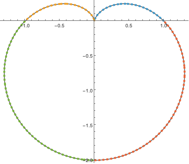
This curve is called a cardioid. In Cartesian coordinates, the cardioid is much more complicated—the implicit equation for the above curve is \((x^2 + y^2)^2 + 2 y (x^2 + y^2) = x^2.\)
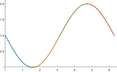
Consider the following functions: \[ f(\theta) = \sin \theta, \qquad f(\theta) = \sin 3 \theta, \qquad f(\theta) = \cos \theta, \quad \text{and} \quad f(\theta) = \cos 2 \theta, \] where all are understood on the domain \(0 \leq \theta \leq 2 \pi\). Which of these match with the following plots?
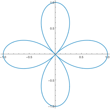
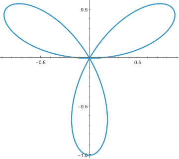
These are called rose curves. Do we really need the entire domain \(0 \leq \theta \leq 2 \pi\) to see the full picture?
Solution
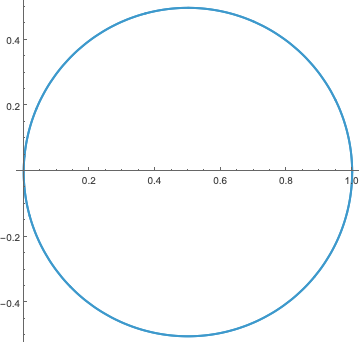
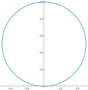
The circle along the \(x\)-axis is \(r = \cos \theta\), while the circle on the \(y\)-axis is \(r = \sin \theta\). Why does the rose curve corresponding to \(r = \sin 3 \theta\) only appear to have three petals, while the one corresponding to \(r =\cos 2 \theta\) has four?
Lines of the form \(y = mx\) can be nicely converted into polar coordinates. Since \(x \tan \theta = y\), the equation \(\tan \theta = m\) defines the line in polar coordinate—usually, one writes \(\theta = \tan^{-1}(m)\). Note that, in this instance, \(r\) is the free variable tracing out the line.
On the other hand, polar coordinates make some simple curves much harder to understand.
Consider the line \(y = mx + b\). Substituting gives \(r \sin \theta = m r \cos \theta + b,\) and solving for \(r\) yields \[ r(\theta) = \frac{b}{\sin \theta - m \cos \theta}, \] which is the polar equation for the line.
If you find this alarming, don’t worry—we aren’t going to use polar coordinates for lines like these! This is a sort of cautionary tale: some coordinates are better suited to certain types of curves than others.
Area element in polar coordinates
In Cartesian coordinates, the area element has a simple form: \(dA = dx \, dy\). We use this impicitly when evaluating double integrals using Fubini’s theorem: \[ \iint_R f(x,y) \, dA = \int_a^b \int_{g_1(x)}^{g_2(x)} f(x,y) \, dy \, dx = \int_c^d \int_{h_1(y)}^{h_2(y)} f(x,y) \, dx \, dy. \]
In polar coordinates, the area element is slightly more complicated: \(dA = r \, dr \, d\theta\).
Hueristically, the \(r\) factor arises because the angle swept out by small changes in \(\theta\) grows as we move away from the origin, so that the increment \(r d\theta\) describes a segment of the region orthogonal to the radial increment \(dr\). See (Stewart, Clegg, and Watson 2020, figs. 15.3.3–4) for a visual explanation.
In particular, note that the naive element \(dr \, d\theta\) has the wrong units!
Write \(R\) for the region enclose by the unit circle. In Cartesian coordinates, we can compute the area by integrating the constant function \(1\): \[ \text{Area}(R) = \int_{-1}^1 \int_{-\sqrt{1-x^2}}^{\sqrt{1-x^2}} dy \, dx = 2 \int_{-1}^1 \sqrt{1-x^2} \, dx. \] In polar coordinates, we integrate over the polar rectangle \(0 \leq r \leq 1\) and \(0 \leq \theta \leq 2\pi\): \[ \text{Area}(R) = \int_0^{2\pi} \int_0^1 r \, dr \, d\theta. \] Which is easier to compute?
If \(f(x,y)\) is a continuous function on a polar rectangle \(\alpha \leq \theta \leq \beta\) and \(a \leq r \leq b\), then \[ \iint_R f(x,y) \, dA = \int_\alpha^\beta \left( \int_a^b f(r \cos \theta, r \sin \theta) \, r \, dr \right) d\theta. \]
Find the volume under \(f(x,y) = x^2+y^2\) and over the annulus \(R\) of inner radius \(1\) and outer radius \(2\):
Solution
Recalling the Pythagorean identity \(x^2 + y^2 = r^2\), we have \[ \iint_R (x^2+y^2) \, dA = \int_0^{2\pi} \int_1^2 r^3 \, dr \, d\theta = \int_0^{2\pi} \left. \frac{r^4}{4} \right|_1^2 d\theta = \int_0^{2\pi} \frac{15}{4} \, d\theta = \frac{15\pi}{2}. \]
Just as in the Cartesian case, we can compute integrals over non-rectangular regions in polar coordinates by introducing bounds for \(r\) in terms of functions of \(\theta\).
Solution
The rightmost petal \(R\) of the rose is given by \(0 \leq r \leq \cos(2\theta)\) and \(-\frac{\pi}{4} \leq \theta \leq \frac{\pi}{4}\). Thus, the area is \[ \text{Area}(R) = \iint_R \, dA = \int_{-\pi/4}^{\pi/4} \int_0^{\cos(2\theta)} r \, dr \, d\theta = \int_{-\pi/4}^{\pi/4} \left. \frac{r^2}{2} \right|_0^{\cos(2\theta)} d\theta = \int_{-\pi/4}^{\pi/4} \frac{\cos^2(2\theta)}{2} d\theta. \] We conclude using the power reduction formula: \[ \text{Area}(R) = \int_{-\pi/4}^{\pi/4} \frac{1 + \cos(4\theta)}{4} d\theta = \left. \frac{\theta}{4} + \frac{\sin(4\theta)}{16} \right|_{-\pi/4}^{\pi/4} = \frac{\pi}{8}. \]
Homework
(Stewart, Clegg, and Watson 2020, sec. 15.3) #1–6, 7, 13, 19, 23